고정 헤더 영역
상세 컨텐츠
본문
AR모형은 t기의 값이 t-k기의 값에 영향을 받는 모형을 말한다
모형의 단순화를 위해
t기의 값이 t-1기의 영향만 받는 모형을 상정하자.
$$ X_{t} = \rho X_{t-1} + \varepsilon_{t} $$
$$ {\varepsilon_{t}} \sim N(0,\sigma^2) $$ , $$ |\rho| <1 $$일때
$$X_{1} = 1 $$
$$X_{2} = \rho $$
$$X_{3} = \rho^2 $$
.
.
.
$$ X_{i} = \rho^{i-1}$$
가 성립하고, 위는 충격반응함수 Impulse Responsive Function(irf)을 의미한다.
t기로 갈수록 rho의 영향을 받아 점점 1기의 충격이 축소됨을 알 수 있다.
매틀랩을 통해 $$\rho=0.1,0.5,0.9$$ 이고, 충격이 매 기 발생하는 3가지 모형을 알아보자
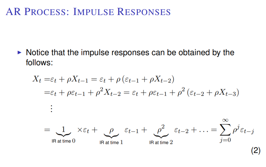
t기에 발생한 충격 $$ \epsilon_{t} $$는 $$ \rho$$의 영향을 받지않아 그대로인 반면,
t-2기에 발생한 충격 $$ \epsilon_{t-2} $$는 $$\rho $$의 영향을 두번 받아 충격이 약화되었다.
$$\rho=1$$ 일때
clc;
format short g;
close all;
clear all;

tic
rand('state',26);
randn('state',26);
ntotal = 200;
nburnin = 100;
nsimper=ntotal-nburnin;
X_0 = 0;


rho=0.1;

shocks=randn(ntotal,1);
X=zeros(ntotal,1);

for i=1:ntotal
    if i==1
        X(i,1)=rho*X_0+ shocks(i,1);
    else
        X(i,1)=rho*X(i-1,1)+ shocks(i,1);
    end
end

X_rho_1=X(nburnin+1:end ,:);

toc

그래프를 살펴보자
전기의 영향 $$\rho$$가 작을수록 norm dist의 평균 0을 크게 이탈하지 않지만,
$$\rho$$가 크면 0을 크게 이탈하는 모습을 보인다
왜냐하면 $$\rho$$가 작을수록 과거 기의 충격이 약화되고, 누적되어도 결국 0에 수렴하게됨으로
t기의 값 $$X_{t}$$는 거의 온전히 t기의 shock $$\epsilon_{t}$$의 영향만 있기 때문이다
( $$\rho$$가 크면 이전 기의 영향이 작아지지 않아 점점 norm dist의 평균 0을 벗어난다 )
%==========================================================================
%
% Mainscript_AR_process.m
% Main file to simulate AR processes
%
%                                        Joonyoung Hur (joonyhur@gmail.com)
%                                    School of Economics, Sogang Univeristy
%==========================================================================

clc;
format short g;
close all;
clear all;

tic

rand('state',26);
randn('state',26);

%% Overall setting
ntotal = 200;               % total number of periods to generate data
nburnin = 100;              % number of periods for initial burn-in
nsimper = ntotal - nburnin;	% number of simulation periods

X_0 = 0;                    % initial value for the AR processes

%% Generate AR process, with rho=0.1
rho = 0.1;  % autocorrelation parameter

shocks = randn(ntotal,1);   % random draws for shocks from the standard normal distribution

X = zeros(ntotal,1);

for i=1:ntotal
    if i==1
        X(i,1) = rho*X_0 + shocks(i,1);
    else
        X(i,1) = rho*X(i-1,1) + shocks(i,1);
    end
end

X_rho_1 = X( nburnin+1:end , :);

%% Generate AR process, with rho=0.5
rho = 0.5;  % autocorrelation parameter

shocks = randn(ntotal,1);   % random draws for shocks from the standard normal distribution

X = zeros(ntotal,1);

for i=1:ntotal
    if i==1
        X(i,1) = rho*X_0 + shocks(i,1);
    else
        X(i,1) = rho*X(i-1,1) + shocks(i,1);
    end
end

X_rho_5 = X(nburnin+1:end,:);

%% Generate AR process, with rho=0.9
rho = 0.9;  % autocorrelation parameter

shocks = randn(ntotal,1);   % random draws for shocks from the standard normal distribution

X = zeros(ntotal,1);

for i=1:ntotal
    if i==1
        X(i,1) = rho*X_0 + shocks(i,1);
    else
        X(i,1) = rho*X(i-1,1) + shocks(i,1);
    end
end

X_rho_9 = X(nburnin+1:end,:);

%% Plot
color0 = rgb('Black');
color1 = rgb('MediumBlue');
color2 = rgb('Crimson');
color3 = rgb('RoyalBlue');
color4 = rgb('ForestGreen');
color5 = rgb('Navy');
color6 = rgb('OrangeRed');
color7 = rgb('Purple');
color8 = rgb('MediumVioletRed');
color9 = rgb('Cyan');
color10 = rgb('Magenta');
color11 = rgb('Lime');
color12 = rgb('LightCyan');
color13 = rgb('HotPink');
color14 = rgb('GreenYellow');
color15 = rgb('Salmon');
color16 = rgb('Gray');
color17 = rgb('LightGray');
color18 = rgb('Gold');
color19 = rgb('DarkGray');
color20 = rgb('DarkCyan');
color21 = rgb('Lavender');
color22 = rgb('LightBlue');
color23 = rgb('LightCoral');

dt = (1:1:nsimper)';

titles = {'AR(1) process with \rho=0.1';
          'AR(1) process with \rho=0.5';
          'AR(1) process with \rho=0.9';
          'AR(1) processes: comparison'};

figure(1)

for ii=1:3
    subplot(3,1,ii)
    if ii==1
        series1 = X_rho_1(:,1);
    elseif ii==2
        series1 = X_rho_5(:,1);
    elseif ii==3
        series1 = X_rho_9(:,1);
    end
    maxvar = 1.01*max(max(series1),max(series1));
    minvar1 = min(series1)-.01*abs(min(series1));
    minvar = min(minvar1,minvar1);
    plot(dt,series1,'-', 'Color', color5, 'MarkerSize',3, 'linewidth',1);
    hold on
    plot(dt,zeros(nsimper,1),'-', 'Color', color0, 'MarkerSize',3, 'linewidth',1);
    hold off
    axis tight
    ylim([minvar maxvar])
    title(char(titles(ii)), 'fontsize', 10);
    grid on
end

figure(1)
set(gcf, 'Units', 'inches');
set(gcf, 'Position', [0 0 9.8 6.3]);
set(gcf, 'renderer', 'painters');
set(gcf, 'PaperPositionMode', 'auto');
% print(gcf, '-depsc2', '-painters', ['ar1_example.eps'])
% close

toc
'코딩일기장 > 통계학' 카테고리의 다른 글
| 회귀분석 Attribute (0) | 2021.12.13 |
|---|---|
| (n-1)s^2/sigma^2 (0) | 2021.11.29 |
| 확률함수 variable transform (0) | 2021.10.22 |
| Moment와 Moment generating function (0) | 2021.10.05 |
| Jensen Inequality (0) | 2021.10.05 |


댓글 영역